Formulation
In order to estimate the motion field we formulate an optimization problem over the state $\mathbf{x}$ for which the camera velocity consistency is imposed as well as those terms corresponding to the pre-integration of the IMU readings. The joint optimization problem will consist on minimizing a cost function $J(\mathbf{x})$ which is the summation of terms associated to the inertial measurements $J_{i}$ as well as to the camera measurements $J_{c}$. Our state estimate $\hat{\mathbf{x}}$ will be the one that minimizing the cost function $J(\mathbf{x})$.
\begin{align} \hat{\mathbf{x}} = min_{\mathbf{x}} J(\mathbf{x}) = min_{\mathbf{x}} \left( J_{c}(\mathbf{x}) + J_{i}(\mathbf{x}) \right) \end{align}As we add more frames, the result is a sliding window of $N$ frames moving along the camera trajectory. In the general case, the cost function $J(\mathbf{x})$ can be expressed compactly using as follows: \begin{equation} J(\mathbf{x})= \sum_{p=i}^{i+N-1}\left(\mathbf{r}_{c_{p}}^\top{\boldsymbol\Sigma}_{c_{p}}^{-1}\mathbf{r}_{c_{p}} + \mathbf{r}_{\Delta \mathbf{v}_{p}}^\top{\boldsymbol\Sigma}_{\Delta \mathbf{v}_{p}}^{-1} \mathbf{r}_{\Delta \mathbf{v}_{p}}\right) + \mathbf{r}_{bg}^\top{\boldsymbol\Sigma}_{\boldsymbol\omega}^{-1} \mathbf{r}_{bg} + \mathbf{r}_{ba}^\top{\boldsymbol\Sigma}_{\mathbf{a}}^{-1} \mathbf{r}_{ba} + \sum_{l=i}^{i+N}\mathbf{r}_{\omega_l }^\top{\boldsymbol\Sigma}_{\boldsymbol\omega}^{-1}\mathbf{r}_{\omega_l} \end{equation} and the state $\mathbf{x} \in \mathbb{R}^{6N+8}$ is defined as: \begin{equation} \mathbf{x} = \left[ {\mathbf{v}}_i^\top,{\boldsymbol\omega}_i^\top,\dots,{\mathbf{v}}_{i+N-1}^\top,{\boldsymbol\omega}_{i+N-1}^\top,{\mathbf{g}}^\top,{\mathbf{b}^g}^\top, {\mathbf{b}^a}^\top \right]^\top \end{equation}
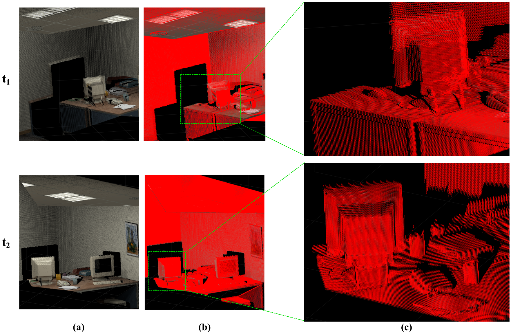
Figure. Motion estimation in an office scene from the ICL-NUIM dataset in two different times t1 and t2. (a) 3D representation of the scene. (b) Motion estimation of the objects in the scene. Every velocity is represented by a red arrow on each point. (c) Zoomed-in areas.
Consider the case in following figure, using a 3-frames-sliding-window. When the $l$-frame comes, the optimization is done. However, in order to keep a 3-frame window, when the next frame $l+1$ comes, we need to marginalize out $\mathbf{v}_i$ and $\boldsymbol{\omega}_i$.
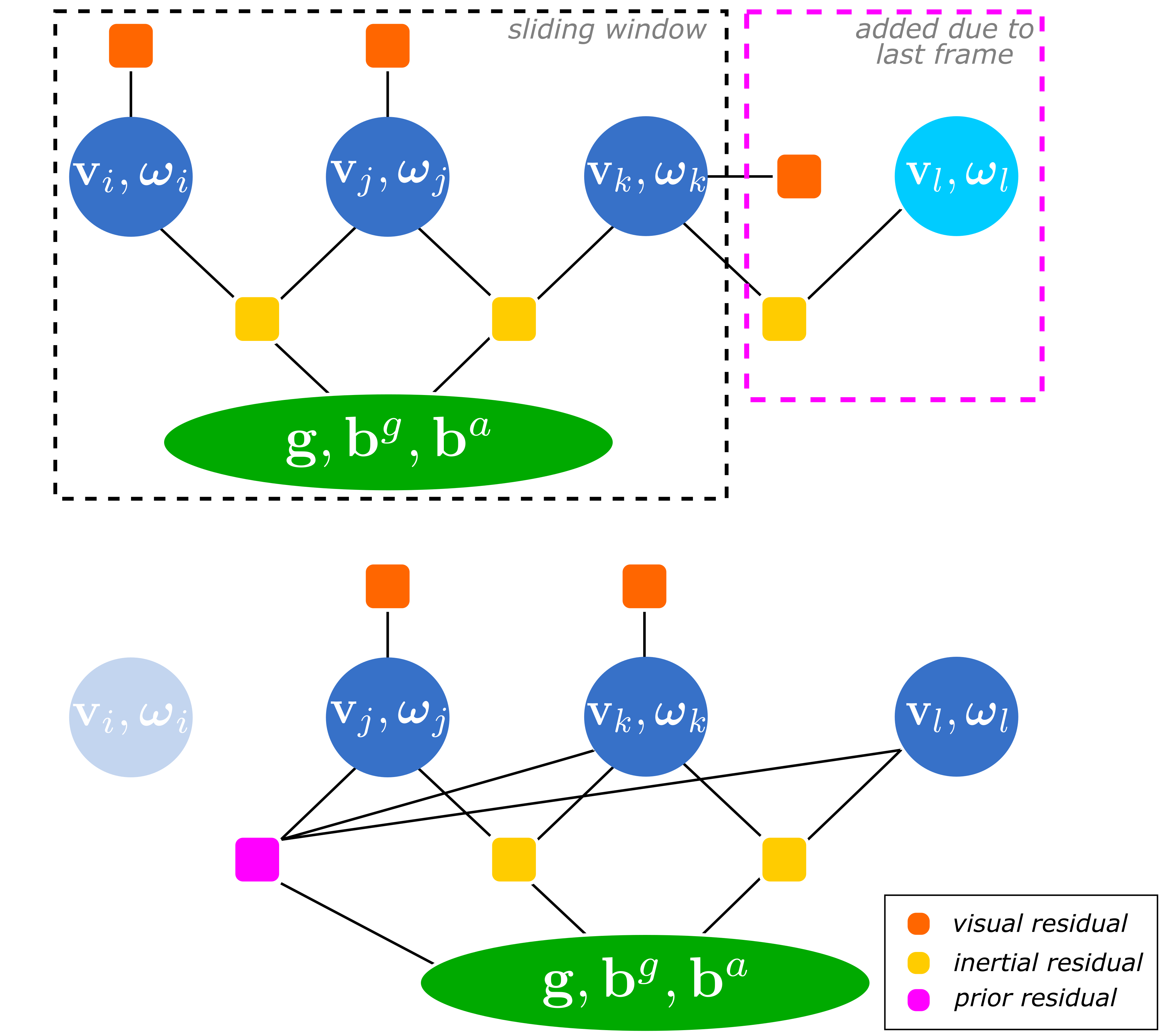
The Hessian $\mathbf{H}$ contains the second derivatives of the cost function with respect to the state variables, that encodes how every state variable affects the others. We denote as $\alpha$ the block of variables we would like to marginalize, and $\beta$ the block of variables we would like to keep. When marginalizing a set $\alpha$ of variables, we gather all factors dependent on them as well as the connected variables $\beta$. This is done by means of the $\textit{Schur Complement}$, which is defined as follows. \begin{equation} \mathbf{H}^* = \mathbf{H}_{\beta\beta} - \mathbf{H}_{\alpha\beta}^\top\mathbf{H}_{\alpha\alpha}^{-1}\mathbf{H}_{\alpha\beta} \end{equation}